F1 2011 Spain Race - Laptime Analysis, WEB and BUT

Some more making-it-up-as-I-go-alongness...

First up, an admission: I'm not much of a statistician.

Second up, a suspicion: I suspect that statisticians have lots of clever trick for using maths and stats to help them tell stories to themselves about the distributions of various populations.

Third up, a vision: that it might be possible to use the tools the statisticians use to get a gut feel about how things are dostributed without having to know too much about the stats, but just doing a bit of common-sense reasoning...

You might say this is an anti-academic view. But then again, my car is blue...* [UPDATE: It's also late, and I've I've come to realise there are a couple of obvious errors in this post that I've tried to highlight...]

* I find this a hilarious response, in much the same way I always laugh to myself about the "What's the differnce between a duck?" joke. The backstory to it is, if anyone asks me what sort of car I have, (let alone how it works) my response is always: "my car's blue"...

So... here's a few ways of looking at Webber's and Button's laptimes. These may or may not be sensible ways - what I'm looking for is ways that might tell us something interesting about how these drivers' racers compared in a purely visual intuitive way (that is, are there visual tools we can throw at the data, and if anything looks vaguely interesting use that as the basis for a more considered look. I'm not suggesting the rash application of tools and measures to find things we might claim. I'm interested in the rash application of tools and measures to see if there's something worth exploring in a little more detail...)

If you'd like to enagage in debate, principled or otherwise, about what if anything, any of the following charts hint at, please feel free to chip in in the comments (I'm making this all up as I go along, and would value corrections as well as other observations/contributions. We're all learning together, right?;-)

First up, a straightforward comparison of laptimes lap-by-lap:



Hmm.. nothing too obvious there, except that they're pitting at different times... How about if we look at fuel corrected laptimes (this shouldn't show much different? Just a compaction of the times perhaps to a smaller range?)



Okay, so the distribution looks sort of flat...so maybe Button has more consistent laptimes than Webber... [UPDATE: arrghhhh GOTCHA moment: the axes are different scales, so the 85s distance on the y-axis is different to the 5s axis on the x axis. Note to self - force them to be the same (err, how do I do this in R? Fixing the range of each axis and the viewing portal to be the same would seem easiest?] that's something we can check - here's the distribution of fuel corrected laptimes plotted explicitly:



And here's the boxplot:



Button is more consistent...

Okay, how about a slightly different sort of scatterplot, specifically, a QQ plot. This works by ranking each driver's laptimes, then plotting the first ranked against the first ranked, the second ranked against the secind ranked, and so on. Two lines are plotted on the chart. One corresponds to x=y. The other line goes through the frst and third quartlie points. First up, by ranked laptime:



Err, erm.. so, err, the lower is x=y, so, err... based on the x=y line: the fastest laps are above the line, so Webber does the fastest fastest laps, in absolute terms. More generally, most of the marks appear below the x=y line, so Button is more consistently on the faster lap? The qqline has a gradient greater than one, and it crosses the x=y line between the first and third quantiles, so, err, erm...? It's late, my intuition is failing me... I'll have to come back to that....

How about the qqplot over the rank ordered fuel corrected laptimes?



(I'm thinking I maybe need to jiggle the axes so the x and y ranges are the same in the above two plots to make for a fairer visual comparison... how'd I set the axis ranges in R then...?)

This time, the qqline gradient is way less than 1, but again the cross seems to appear between first and third quartiles, so, err... erm... it's late, I'm slow tonight...?:-(

Should I maybe try a best fit line as well? How do I do that in R?

As far as the pitstop times go, because the drivers did different startegies (3 stop for BUT vs 4 for WEB) I'm not sure we can do much of a comparison (unless we compare slowest 3 stops... For a more literal comparison, see the F1 2011 Spain Race - Pit Stop Analysis.)

Assuming that when I come to the qqline/quartile line with a clear head I can make some sense of it, here's a quick look at the ranked fuel corrected laptimes for Hamilton and Vettel:



Recalling that in F1 2011 Spain Race - Driver Comparisons I couldn't really identify who was "faster", the closeness of the two lines in the above plot suggests the drivers were pretty evenly matched?

Note: I couldn't get the qqline() R function to work, (it wouldn't plot anything?) but instead I found this function:
qqline2 <- function (x, y, ...)
{
y <- quantile(y[!is.na(y)], c(0.25, 0.75))
x <- quantile(x[!is.na(x)], c(0.25, 0.75))
slope <- diff(y)/diff(x)
int <- y[1L] - slope * x[1L]
abline(int, slope, ...)

The lines were then plotted using the commands:
qqline2(WEB$fuelCorrectedLaptime,BUT$fuelCorrectedLaptime)
abline(0,1)

F1 2011 Spain Race - Pit Stop Analysis

One of the things I've started trying to pull together is a "comprehensive" spreadsheet organised by lap-and-driver containing all sorts of data grabbed directly from FIA timing sheets and also derived from that data (see the Data page for links).

This mega-spreadsheet can then been re-mined to produce all sorts of different reports.

So for example, here's the pitstop times for each driver during the Spanish Grand Prix:



(The columns in this table are sortable; click on a column header to sort by that column.)

The essential data for this table was grabbed from the Comprehensive data sheet using a pivot table of the form:



Howto embed the interactive table: View Source to see how I embedded the interactive table using data pulled dynamically from a Google spreadsheet.

F1 2011 Spain Race - Driver Comparisons

Here's a handful of laptime comparisons between drivers displayed using a QQplot. These plots are generated by ranking each drivers laptime, then pltting the first ranked time of one driver against the first ranked time of the second driver, the second ranked time against the second ranked time, and so on.

The line in the plot is x=y. If the trace falls below this line, it shows the driver on the y-axis has a faster time. Conversely, if the plots are above the line, the driver on the x-axis was faster on those rank-ordered laps.

Here's how Hamilton and Button compare:



We see how the Hamilton's laps, ordered in terms of duration, are considerably faster than Button's ordered laptimes. But, as I suggest below, this sort of laptime comparison may be misleading...

How about Vettel and Hamilton, given the race was closely fought between these two drivers?



If we look closely at this it seems that for many of the early laps, the marks are below the line, which is to say, Hamilton has the upperhand in terms of speed? Again, this may be misleading...

Nevertheless, let's zoom in on this, and omit the pitstops;



Hamilton definitely appears to have faster faster laps (sic) than Vettel. But - and here is the but that I hinted at before that maybe renders the above charts a bit misleading - maybe the fuel weight penalty is affecting things?

For example, when the ranking is calculated, the Nth ranked lap for Vettel may be from lap 4 of the race, compared to lap 44 for Hamilton. If we instead look at fuel corrected laptimes, then we're ranking laps based on "pure speed", with the fuel weight penalty affect on laptime accounted form (essentially, I'm trying to "normalise" the laptimes so that lap order doesn't play a role). What happens to the QQplot then? Here's a plot of ranked fuel corrected laptimes for Hamilton and Vettel:



Here, we see that the very fastest fuel corrected lap times go to Vettel, but then there are a few highly ranked fuel corrected times from Hamitlon. Does a change of symbol type help us see things and more clearly?



For times under about 86.5s, I think Hamilton has it? But in general, I'm not sure (form these charts) that we can say whether or not Hamilton of Vettel was generally faster? (See also the fuel corrected laptime comparison by lap).

Here's a really badly laid out scatterplot showing their fuel corrected laptimes compare:




Note: here are some R cribs for generating these charts:

VET<-subset(esp_2011stintLapTimes, car==1) //define a subset of the original CSV data
HAM<-subset(esp_2011stintLapTimes, car==3)
qqplot(VET$fuelCorrectedLaptime,HAM$fuelCorrectedLaptime,main="Driver comparison chart: VET and HAM",xlab="VET (ranked fuel corrected laptimes(s))",ylab="HAM (ranked fuel corrected laptimes(s))")
abline(0,1) //plots the x=y line
VET<-subset(esp_2011stintLapTimes, car==1 & lapTime<95) //a clunky way fo doing the zoom in to the data
HAM<-subset(esp_2011stintLapTimes, car==3 & lapTime<95)
qqplot(VET$fuelCorrectedLaptime,HAM$fuelCorrectedLaptime,main="Driver comparison chart: VET and HAM",xlab="VET (ranked fuel corrected laptimes(s))",ylab="HAM (ranked fuel corrected laptimes(s))",pch=3) //pch= sets the symbol type
abline(0,1)

F1 2011 Spain Race - Stint Comparison

Here's how the drivers compared with respect to stints (that is, how many laps each driver did per stint during the 2011 F1 Spanish Grand Prix):



Here's the data:

F1 2011 Spain Race - Fuel Corrected Laptime Comparisons

A quick comparison of the fuel corrected laptimes between Hamilton and Vettel:



(You can find the data here: Stint laptimes data.)

And here's how the times compare for Hamilton and Button:

F1 2011 Spain Race - Race History According to Alonso

A quick plot showing a variant of race history, specifically the time elapsed time difference at each lap between Alonso and the other cars:



You can get the data used to generate this plot from F1 2011 Spain: Elapsed Time Data

F1 2011 Spain Free Practice - Tyres

One of the things I want to start exploring is whether or not there's enough in the practice laptimes data for the armchair strategist to play with when it comes to getting a feel for how the race might play out and what sorts of strategies might be relevant.

So here's a first attempt looking at some of the fuel corrected laptimes over some long practice stints for one or two of the drivers. (Timing data available here. Fuel time correction data obtained from AT&TWIlliams: Spanish GP Preview.)

To start with, let's look at Mark Webber (WEB). Here's how Red Bull made use of the practice sessions - the time along the bottom is the elapsed time of the particular session in seconds starting from the first mark on the timing sheet by any driver. The colours denote practice session (first, second or third free practice) and the symbols identify different stints. I've oopsed badly on the labelling of the y-axis: it's actually fuel corrected laptimes (about fuel corrected laptimes):



We see the long stint, red FP2 times do appear to be showing a drop off in time (remember, these are fuel weight penalty adjusted times) over each stint.

So you can get a feel for reading the chart, here's Red Bull's session utilisation chart for free practice 2 (WEB's laps are inside the circle); the chart is read like an elapsed time clock across the session.



Looking at other session utilisation charts, I noticed that Alguesuari seemed to have a long FP2 stint, so let's look at his times:



After an initial coming of of the tyres (maybe?) at the start of the long stint at the end of FP2, do the tyres hang on pretty well (with maybe only a slight fade) before the raggedy times at the end of the stint?

Let's take a closer look:



At this scale, we might say the fade isn't that much. But closer up?



A definite drop off - on the order of a tenth of a second per lap. But there seems to be structure in those times two - so have I made a systematic error in my fuel adjustment calculations, or was ALG doing an on/off, this way/that way trial of some sort over those few laps?

Looking at Renault's FP2 session utiisation chart, Petrov's times are interesting, Towards the end of the session, did he maybe try a pitstop?



Here are his laptimes over all three sessions:



And here's a close-up on the long stint at the end of FP2:



Do the tyres start to go off around 4200s? (Remember, the fuel weight adjustment is approximate...) Do we see a pitstop around 4750s and resulting improvement in laptime from a fresh pair of tyres around the 5000s elapsed time mark?

Commands for generating the scatterplots (R-Studio) - of the form:

t='F1 2011 - Spain: Free Practice: KOV'
dnum='20'
plot(Fuel.Corrected.Laptime ~ Elapsed,data=subset(esp_2011practicelaptimes,DriverNum==dnum ),pch=Stint,col=Session, main=t,xlab="Elapsed Time",ylab="Fuel Corrected Laptime (s)")
legend(4000,109,c("FP1","FP2","FP3"),col=1:3,pch=1:1:1)

PS here's another view - long stint times across all drivers/all sessions:

F1 2011 Spain Qualifying

Reports from qualifying, including session participation and lap time distributions. (Get the data here.)

For starters, how the teams utilised qualifying:



(Arghh - a gremlin has snuck in in the inner circle labelling... but i'm not minded to go hunting it down right now...:-(]

And here are the laptime distributions, as a scatterplot:



and as a boxplot:



You can find the data here:

F1 2011 Spain Free Practice - Timing Data

Here's a link to a spreadsheet containing the timing data from the three free practice sessions: F1 2011 Spain - Free Practice Timing Data

Columns included:

• Session (i.e. FP1, FP2 or FP3)


• Name (name of driver)


• DriverNum (the car/driver number)


• Lap (the lap number, corresponding to separate times on timing sheet)


• Time (laptime)


• Elapsed (elapsed time in the session, in seconds, as counted from the first time appearing on the timing sheet)


• Stint (the stint number, identified according to the heuristics described below)


• Fuel Corrected Laptime (that is, fuel weight penalty corrected laptime within that stint)


• Stint Length (the number of laps in the stint)


• Lap in stint (the lap number within the stint)

The heuristic used to identify stints is:
- ignore first "lap" time on timing sheet for each driver;
- end of stint if laptime > 1.5* fastest laptime in that session for that driver



If you do any visualisations/analysis of the data anywahere:
- please post a link in the comments to any related blog posts you publish
- please let me know if you'd like to post your visualisation/analysis on this blog:-)

F1 2011 Spain Free Practice - Laptime Distributions

A visual summary of laptime distributions

(Note that laptimes exceeding 1.5 times the time of a driver's fastest lap are not shown.)















The R commands used to generate these images are of the form:

plot(Time ~ DriverNum,data=esp_2011p3laptimes, main='F1 2011 - Spain: Free Practice 3',xlab="Car",ylab="Laptime (s)")

and

boxplot(Time ~ DriverNum,data=esp_2011p3laptimes, main='F1 2011 - Spain: Free Practice 3',xlab="Car",ylab="Laptime (s)")

PS here's a better R recipe for plotting charts with driver name labels:

//set font size
par(ps=15)
plot(Time ~ DriverNum,data=esp_2011p3laptimes, main='F1 2011 - Spain: Free Practice 3',xlab="Driver",ylab="Laptime (s)",xaxt='n')
labels=c("VET","WEB","HAM","BUT","ALO","MAS","SCH","ROS","HEI","PET","BAR","MAL","","SUT","RES","KOB","PER","BUE","ALG","TRU","KOV","KAR","LIU","GLO","AMB")
//set font size
par(ps=10)
text(1:25,par("usr")[3],srt=90,adj=1,labels=labels,xpd=TRUE)

F1 2011 Spain Free Practice 3 - Utilisation

Here's a graphical summary of how the teams made use of the time available in FP3:

F1 2011 Spain Free Practice 2 - Utilisation

How the teams made use of second free practice...

F1 2011 Spain Free Practice 1 - Utilisation

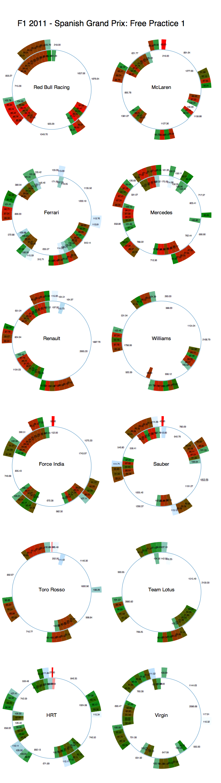
A quick overview of how the teams made use of Free Practice 1. Session time progresses round the donut with a start time corresponding to the earliest time recorded on the timing sheet, and the end time corresponding to the time the final recorded time. Each team's graphic shows the activity of both drivers, with driver 1 on the outside and driver 2 on the inside. Segments get hotter/redder the faster they are (I need to find out how to suppress the colour in the first segment - the time to emergence (that is, the time in seconds the car appeared after the appearance of the first car on the timing sheet).




A quick glimpse over the chart as a whole show the Red Bulls appear to be in good form, along with Massa and maybe even the Mercedes?